无平衡点分数阶混沌系统全状态自适应控制

引用本文

邵克勇, 陈丰, 王婷婷, 王季驰, 周立朋. 无平衡点分数阶混沌系统全状态自适应控制. 2017, 47(4): 1225-1230
SHAO Ke-yong, CHEN Feng, WANG Ting-ting, WANG Ji-chi, ZHOU Li-peng. Full state based adaptive control of fractional order chaotic system without equilibrium point. Journal of Jilin University Engineering and Technology Edition, 2017, 47(4): 1225-1230 复制到剪切板

Permissions

无平衡点分数阶混沌系统全状态自适应控制

邵克勇, 陈丰, 王婷婷, 王季驰, 周立朋

东北石油大学电气信息工程学院,黑龙江大庆 163318

作者简介:邵克勇(1970-),男,教授,博士.研究方向:鲁棒控制,智能控制.E-mail:1127073951@qq.com

基金:东北石油大学研究生创新科研项目(YJSCX2015-032NEPU,YTSGX2015-031NEPU).

摘要

针对一类无平衡点的分数阶混沌系统,首先通过分数阶微分变换方法(FDTM)得到它的解序列。然后,研究了系统的Kaplan-Yorke维数和耗散性,基于系统的离散映射通过QR分解得到最大Lyapunov特征指数,通过该特征指数可以判断系统是否保持混沌。最后,给出一种全状态自适应控制方法,使系统的状态变量追踪期望轨迹,并通过数值模拟验证了本文算法的可行性。

关键词: 自动控制技术; 人工智能; 无平衡点的混沌系统; 分数阶微分变换方法; 全状态自适应控制; Lyapunov特征指数

中图分类号:TP273 文献标志码:A 文章编号:1671-5497(2017)04-1225-06

Full state based adaptive control of fractional order chaotic system without equilibrium point

SHAO Ke-yong, CHEN Feng, WANG Ting-ting, WANG Ji-chi, ZHOU Li-peng

College of Electrical Engineering and Information, Northeast Petroleum University, Daqing 163318,China

Abstract

For a class of chaotic system without equilibrium point, its solution series is obtained by the Fractional Differential Transformation Method (FDTM). Then, the Kaplan-Yorke dimension and the dissipativity of the system are investigated. The Lyapunov characteristic exponents are calculated based on the discrete map of the system through QR factorization algorithm, and the largest Lyapunov characteristic exponent is applied to judge whether the system keeps chaos or not. Finally, a full state based adaptive controller for the fractional order chaotic system is designed, which allows the states of the system to track the desired constant. The feasibility of the proposed algorithm is verified by numerical simulation.

Keyword: automatic control technology; artificial intelligence; chaotic system without equilibrium point; fractional differential transformation method(FDTM); full state based adaptive control; Lyapunov characteristic exponent

Show Figures

0 引言

分数阶系统是包含分数阶积分与微分的动态系统, 它可以有效地应用于物理系统建模^{[1, 2, 3]}。在整数阶微积分的意义下, Poincare-Bendixon定理指出:连续自治系统出现混沌现象的微分阶次必须大于等于3^{[4, 5]}。但是, 人们在研究中发现, 在分数阶微积分的意义下, 在许多阶次低于3的分数阶非线性系统中, 仍然存在混沌现象^[6]。由于分数阶混沌系统相比于整数阶具有更好的发展前景, 它的理论研究及实际应用受到国内外学者的普遍关注。然而该领域内的研究成果仍然偏少, 其中一个主要原因是分析非线性分数阶系统稳定性的理论工具具有局限性。文献^[7]提出了基于线性分数阶系统稳定性理论的混沌控制方法, 然而这种方法只验证了局部的稳定性。文献^[8]提出了主动控制的方法, 这种方法利用非线性控制律来消除控制系统中的非线性项, 再根据线性分数阶系统稳定性理论, 设计一个线性控制律来稳定此系统, 但当系统中的参数未知时, 不能用主动控制方法来设计控制器。文献^[9]研究了一类整数阶新型金融系统的自适应控制。文献^{[10, 11]}研究了分数阶混沌系统的自适应控制, 其中控制变量存在于局部系统方程中。

本文针对一类无平衡点的分数阶混沌系统, 设计了一种全状态自适应控制器, 在不消除非线性项的情况下来追踪期望轨迹。最后通过数值模拟, 验证了该算法的可行性。

1 预备知识

本节给出了分数阶微积分和微分变换方法的一些定义和性质^[12]。

1.1 分数阶微积分

$\begin{matrix} _{t_{0}} D_{t}^{q} \end{matrix}$ 表示分数阶微分积分算子。当 $\begin{matrix} q \end{matrix}$ 为正值时, 它是一个微分算子; 当 $\begin{matrix} q \end{matrix}$ 为负值时, 它是一个积分算子。分数阶微分的定义通常用Grunwald-Letnikov, Riemann-Liouville和Caputo来表示。

$\begin{matrix} _{t_{0}} D_{t}^{q} ≜ D_{t}^{q} = \{\begin{matrix} \frac{d^{q}}{d t^{q}}, q > 0 \\ 1, q = 0 \\ {\int_{t_{0}}^{t} (dτ)}^{q} ≜ I^{- q}, q < 0 \end{matrix} (1) \end{matrix}$

Riemann-Liouville定义^[13], 表示如下:

$\begin{matrix} _{t_{0}} D_{t}^{q} f (t) = \frac{1}{Γ (1 - q)} \frac{d}{dt} \int_{0}^{t} \frac{f (τ)}{{(t - τ)}^{q - n + 1}} dτ (2) \end{matrix}$

式中: $\begin{matrix} n - 1 < q < n; Γ (\cdot) \end{matrix}$ 是Gamma函数。

根据方程(1)(2), 分数阶微分和积分算子的阶次为 $\begin{matrix} 0 < q < 1, t_{0} = 0 \end{matrix}$ (本文始终考虑 $\begin{matrix} t_{0} = 0 \end{matrix}$ 的情况), 并且分别定义为:

$\begin{matrix} \begin{matrix} _{0} D_{t}^{q} {f (t) = \frac{1}{Γ (1 - q)} \frac{d}{dt} \int_{0}^{t} (t - τ)}^{- q} f (τ) dτ \\ _{0} I_{t}^{q} {f (t) = \frac{1}{Γ (q)} \frac{d}{dt} \int_{0}^{t} (t - τ)}^{q - 1} f (τ) dτ \end{matrix} \end{matrix}$

由此, 可以得到 $\begin{matrix} _{0} D_{t}^{q} = \frac{d}{dt} (_{0} I_{t}^{1 - q}) 。 \end{matrix}$

选择Caputo求解分数阶微分方程的重要原因是它对常数求导结果为0, 然而Riemann-Liouville分数阶微分对常数求导结果不恒为0。

1.2 微分变换方法

函数 $\begin{matrix} f (t) \end{matrix}$ 依据分数阶幂级数展开为:

$\begin{matrix} f (t) = \overset{\infty}{\sum_{k = 0}} F (k) {(t)}^{kq} (3) \end{matrix}$

式中: $\begin{matrix} 0 < q < 1 \end{matrix}$ 为分数阶微分的阶次; $\begin{matrix} F (k) \end{matrix}$ 是 $\begin{matrix} f (t) \end{matrix}$ 的分数阶微分变换, 表示如下:

$\begin{matrix} F (k) = \frac{1}{Γ (qk + 1)} {(_{0} D_{t}^{q})}^{k} (f (0)) (4) \end{matrix}$

式中: 是k次可微Caputo分数阶微分。

近似函数 $\begin{matrix} f (t) \end{matrix}$ 为:

$\begin{matrix} f (t) = \overset{N}{\sum_{k = 0}} F (k) {(t)}^{kq} (5) \end{matrix}$

以下是Caputo分数阶微分变换的基本性质^[14]:①如果f(t)=g(t)± h(t), 则F(k)=g(k)± H(k); ②如果f(t)=g(t)h(t), 则F(k)= $\begin{matrix} \overset{k}{\sum_{m = 0}} \end{matrix}$ G(m)H $\begin{matrix} (k - m) \end{matrix}$ ; ③如果 $\begin{matrix} f (t) =_{0} D_{t}^{q} g (t), \end{matrix}$ 则 $F (k) = \frac{Γ (q (k + 1) + 1)}{Γ (qk + 1)} G (k + 1)$ 。

对于分数阶系统来说, 最常用的方法是用时间序列重构相空间, 计算最大Lyapunov指数^[15], 这种做法仍有很多缺点, 如难以选择嵌入维数以及相空间重构的固有延迟参数^[16]。本文利用FDTM得到一组分数阶微分方程的解, 用于计算分数阶系统中的Lyapunov特征指数。

引理1^[17] 设 $\begin{matrix} x (t) \in R^{n} \end{matrix}$ 是一个可微函数, 对于任意 $\begin{matrix} t \geq 0 \end{matrix}$ 时, 存在以下关系:

$\begin{matrix} \begin{matrix} _{0} D_{t}^{q} (x^{T} (t) Px (t)) / 2 \leq x^{T} (t) P_{0} D_{t}^{q} x (t) (6) \\ \forall q \in (0, 1) \end{matrix} \end{matrix}$

式中: $\begin{matrix} P \in (R^{n \times n}) \end{matrix}$ 为常数正定对称矩阵。

定理1^{[18, 19]} 设 $\begin{matrix} x (t) = 0 \end{matrix}$ 为系统的一个平衡点, 且:

$\begin{matrix} _{0} D_{t}^{q} x (t) = f (t, x (t)) (7) \end{matrix}$

假设存在一个Lyapunov函数 $\begin{matrix} V (t, x) 和一个 k 级函数 γ_{i} (i = 1, 2, 3) \end{matrix}$ 满足:

$\begin{matrix} \begin{matrix} γ_{1} (‖ x (t) ‖) \leq V (t, x) \leq γ_{2} (‖ x (t) ‖) \\ _{0} D_{t}^{q} V (t, x) \leq - γ_{3} (‖ x (t) ‖) (8) \end{matrix} \end{matrix}$

式中: $\begin{matrix} q \in (0, 1), \end{matrix}$ 则系统(7)是渐近稳定的。

2 主要结论

提出一个分数阶系统方程:

$\begin{matrix} \{\begin{matrix} _{0} D_{t}^{q} x_{1} = x_{2} \\ _{0} D_{t}^{q} x_{2} = x_{3} \\ _{0} D_{t}^{q} x_{3} = c_{1} x_{2} + c_{2} x_{1} x_{3} + c_{3} x_{2} x_{3} + c_{4} \end{matrix} (9) \end{matrix}$

式中: $\begin{matrix} _{0} D_{t}^{q} \end{matrix}$ 是初始状态 $\begin{matrix} t_{0} = 0 、 \end{matrix}$ 系统的参数为 $\begin{matrix} c_{i} \neq 0 (i = 1, 2, 3, 4) 、 \end{matrix}$ 阶次为 $\begin{matrix} q \in (0, 1) \end{matrix}$ 的Caputo分数阶算子。

2.1 系统特性

2.1.1 平衡点

由于系统方程(9)在 $\begin{matrix} c_{4} \neq 0 \end{matrix}$ 时无平衡点, 因此不能通过Jacobi矩阵的特征值确定系统混沌阶数 $\begin{matrix} q \end{matrix}$ 的范围。

2.1.2 分数阶Lyapunov维数和耗散性

选择参数:c₁=1; c₂=1; c₃=1; c₄=0.75; q=0.95。这个系统的差分变换为:

$\begin{matrix} \{\begin{matrix} \frac{Γ (q (k + 1) + 1)}{Γ (qk + 1)} X_{1} (k + 1) = X_{2} (k) \\ \frac{Γ (q (k + 1) + 1)}{Γ (qk + 1)} X_{2} (k + 1) = X_{3} (k) \\ \frac{Γ (q (k + 1) + 1)}{Γ (qk + 1)} X_{3} (k + 1) = - X_{2} (k) - \\ \overset{k}{\sum_{m = 0}} X_{1} (m) X_{3} (k - m) - \\ \overset{k}{\sum_{m = 0}} X_{2} (m) X_{3} (k - m) - 0.75 \end{matrix} (10) \end{matrix}$

$\begin{matrix} n \end{matrix}$ 阶逆变换的解为:

$\begin{matrix} \{\begin{matrix} x (t) = \overset{N}{\sum_{m = 0}} X (m) {(t - t_{0})}^{mα} \\ y (t) = \overset{N}{\sum_{m = 0}} Y (m) {(t - t_{0})}^{mα} \\ z (t) = \overset{N}{\sum_{m = 0}} Z (m) {(t - t_{0})}^{mα} \end{matrix} (11) \end{matrix}$

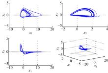
选取时间间隔Δ t=0.01、N=4, 混沌吸引子的相图如图1所示。

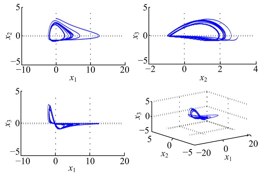	Figure Option View Download New Window
	图1 混沌吸引子的相图Fig.1 Phase portraits of chaotic attractor

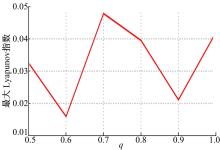
利用文献^[20]中提到的方法, 令L₁=0.012, L₂=-0.0124, L₃=-3.6386, L₁+L₂+L₃=-3.6390< 0。根据Kaplan Yorke猜想, 定义系统(9)的分数阶Lyapunov维数^[21]如下:

$\begin{matrix} D_{KY} = S + \frac{\overset{s}{\sum_{i = 1}} L_{i}}{|L_{s} + 1|} \end{matrix}$

式中: $\begin{matrix} \overset{s}{\sum_{i = 1}} \end{matrix}$ L_i> 0, $\begin{matrix} \overset{s + 1}{\sum_{i = 1}} \end{matrix}$ L_i< 0; L_i(i=1, 2, …, n)是系统(9)的Lyapunov指数; $\begin{matrix} S \end{matrix}$ 为最大整数。显然, 如果其中一个Lyapunov指数是正定的, 并且它们的总和是负的, 则系统(9)是混沌和耗散的。另外, 该系统的Kaplan-Yorke维度是D_KY=1.9677。如图2所示, 当q∈ [0.5, 1]时, 得出最大的Lyapunov指数, 且大于零, 则表示该系统是混沌的。

	Figure Option View Download New Window
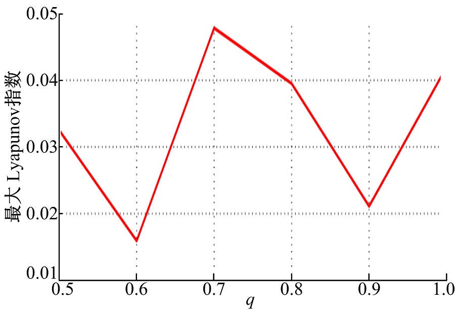	图2 随q变化的最大Lyapunov指数曲线Fig.2 Largest Lyapunov exponent curve versus q

2.2 分数阶系统的自适应控制

受控的分数阶混沌系统为:

$\begin{matrix} \{\begin{matrix} _{0} D_{t}^{q} x_{1} = x_{2} + u_{1} (x) \\ _{0} D_{t}^{q} x_{2} = x_{3} + u_{2} (x) \\ _{0} D_{t}^{q} x_{3} = c_{1} x_{2} + c_{2} x_{1} x_{3} + c_{3} x_{2} x_{3} + c_{4} + u_{3} (x) \end{matrix} (12) \end{matrix}$

式中: $\begin{matrix} x^{Τ} = (x_{1}, x_{2}, x_{3}) 。 \end{matrix}$

假设:

$\begin{matrix} \{\begin{matrix} u_{1} (x) = K_{1} x \\ u_{2} (x) = K_{2} x \\ u_{3} (x) = K_{3} x + {\hat{U}}_{3} (x) \end{matrix} (13) \end{matrix}$

式中: $\begin{matrix} K_{i} = (k_{i, 1}, k_{i, 2}, k_{i, 3}), i = 1, 2, 3 。 \end{matrix}$ 可以得出

$\begin{matrix} \{\begin{matrix} _{0} D_{t}^{q} x_{1} = x_{2} + k_{1, 1} x_{1} + k_{1, 2} x_{2} + k_{1, 3} x_{3} \\ _{0} D_{t}^{q} x_{2} = x_{3} + k_{2, 1} x_{1} + k_{2, 2} x_{2} + k_{2, 3} x_{3} \\ _{0} D_{t}^{q} x_{3} = c_{1} x_{2} + c_{2} x_{1} x_{3} + c_{3} x_{2} x_{3} + c_{4} + \\ k_{3, 1} x_{1} + k_{3, 2} x_{2} + k_{3, 3} x_{3} + {\hat{U}}_{3} (x) \end{matrix} (14) \end{matrix}$

研究了使得系统的状态x₁ 、x₂ 、x₃ 达到常数r₁ 、r₂ 、r₃ 的控制器u₁ (x)、u₂ (x)、u₃ (x)设计问题。

设控制误差为:

$\begin{matrix} \{\begin{matrix} e_{1} (t) = x_{1} - r_{1} \\ e_{2} (t) = x_{2} - r_{2} \\ e_{3} (t) = x_{3} - r_{3} \end{matrix} (15) \end{matrix}$

则动态误差为:

$\begin{matrix} \{\begin{matrix} _{0} D_{t}^{q} e_{1} (t) = (e_{2} (t) + r_{2}) + k_{1, 1} (e_{1} (t) + r_{1}) + \\ k_{1, 2} (e_{2} (t) + r_{2}) + k_{1, 3} (e_{3} (t) + r_{3}) \\ _{0} D_{t}^{q} e_{2} (t) = (e_{3} (t) + r_{3}) + k_{2, 1} (e_{1} (t) + r_{1}) + \\ k_{2, 2} (e_{2} (t) + r_{2}) + k_{2, 3} (e_{3} (t) + r_{3}) \\ _{0} D_{t}^{q} e_{3} (t) = c_{1} (e_{2} (t) + r_{2}) + c_{2} (e_{1} (t) + r_{1}) \\ (e_{3} (t) + r_{3}) + c_{3} (e_{3} (t) + r_{3}) (e_{3} (t) + r_{3}) + \\ k_{3, 1} (e_{1} (t) + r_{1}) + k_{3, 2} (e_{2} (t) + r_{2}) + \\ k_{3, 3} (e_{3} (t) + r_{3}) + c_{4} + {\hat{U}}_{3} (x) \end{matrix} (16) \end{matrix}$

式中: $\begin{matrix} r_{i} (i = 1, 2, 3) \end{matrix}$ 为任意常数。

为了简便, 假设 $\begin{matrix} r_{i} = 0 (i = 1, 2, 3), \end{matrix}$ 由式(16), 得:

$\begin{matrix} \{\begin{matrix} _{0} D_{t}^{q} e_{1} (t) = e_{2} (t) + k_{1, 1} e_{1} (t) + k_{1, 2} e_{2} (t) + \\ k_{1, 3} e_{3} (t) \\ _{0} D_{t}^{q} e_{2} (t) = e_{3} (t) + k_{2, 1} e_{1} (t) + k_{2, 2} e_{2} (t) + \\ k_{2, 3} e_{3} (t) \\ _{0} D_{t}^{q} e_{3} (t) = c_{1} e_{2} (t) + c_{2} e_{1} (t) e_{3} (t) + \\ c_{3} e_{2} (t) e_{3} (t) + k_{3, 1} e_{1} (t) + k_{3, 2} e_{2} (t) + \\ k_{3, 3} e_{3} (t) + c_{4} + {\hat{U}}_{3} (x) \end{matrix} (17) \end{matrix}$

定理2 设计一个自适应控制器为:

$\begin{matrix} \{\begin{matrix} u_{1} (x) = K_{1} x \\ u_{2} (x) = K_{2} x \\ u_{3} (x) = K_{3} x + {\hat{U}}_{3} (x) \end{matrix} (18) \end{matrix}$

式中: $\begin{matrix} {\hat{U}}_{3} (x) = - {\hat{c}}_{1} (t) x_{2} (t) - {\hat{c}}_{2} (t) x_{1} (t) x_{3} (t) - {\hat{c}}_{3} x {(t)}_{2} (t) x_{3} (t) - {\hat{c}}_{4} (t), \end{matrix}$ 选取参数自适应律为:

$\begin{matrix} \{\begin{matrix} _{0} D_{t}^{q} {\hat{c}}_{1} (t) = x_{2} (t) x_{3} (t) \\ _{0} D_{t}^{q} {\hat{c}}_{2} (t) = x_{2} (t) x_{3}^{2} (t) \\ _{0} D_{t}^{q} {\hat{c}}_{3} (t) = x_{2} (t) x_{3}^{2} t) \\ _{0} D_{t}^{q} {\hat{c}}_{4} (t) = x_{3} (t) \end{matrix} (19) \end{matrix}$

如果满足以下条件:

$\begin{matrix} [\begin{matrix} k_{1, 1} \\ k_{2, 1} \\ k_{2, 1} \end{matrix} \begin{matrix} k_{1, 2} + 1 \\ k_{2, 2} \\ k_{3, 2} \end{matrix} \begin{matrix} k_{1, 3} \\ k_{2, 3} + 1 \\ k_{3, 3} \end{matrix}] < 0 \end{matrix}$

则系统(12)是渐近稳定的。

证明误差动态方程为:

$\begin{matrix} \{\begin{matrix} _{0} D_{t}^{q} e_{1} (t) = e_{2} (t) + k_{1, 1} e_{1} (t) + k_{1, 2} e_{2} (t) + \\ k_{1, 3} e_{3} (t) \\ _{0} D_{t}^{q} e_{2} (t) = e_{3} (t) + k_{2, 1} e_{1} (t) + k_{2, 2} e_{2} (t) + \\ k_{2, 3} e_{3} (t) \\ _{0} D_{t}^{q} e_{3} (t) = (c_{1} - {\hat{c}}_{1} (t)) e_{2} (t) + (c_{2} - {\hat{c}}_{2} (t)) \times \\ e_{1} (t) e_{3} (t) + (c_{3} - {\hat{c}}_{3} (t)) e_{2} (t) e_{3} (t) + \\ k_{3, 1} e_{1} (t) + k_{3, 2} e_{2} (t) + k_{3, 3} e_{3} (t) + (c_{4} - {\hat{c}}_{4} (t)) \end{matrix} (20) \end{matrix}$

参数估计误差定义为

$\begin{matrix} \{\begin{matrix} e c_{1} (t) = c_{1} - {\hat{c}}_{1} (t) \\ e c_{2} (t) = c_{2} - {\hat{c}}_{2} (t) \\ e c_{3} (t) = c_{3} - {\hat{c}}_{3} (t) \\ e c_{4} (t) = c_{4} - {\hat{c}}_{4} (t) \end{matrix} (21) \end{matrix}$

根据分数阶的性质, 可以得到:

$\begin{matrix} \{\begin{matrix} _{0} D_{t}^{q} e c_{1} (t) = -_{0} D_{t}^{q} {\hat{c}}_{1} (t) \\ _{0} D_{t}^{q} e c_{2} (t) = -_{0} D_{t}^{q} {\hat{c}}_{2} (t) \\ _{0} D_{t}^{q} e c_{3} (t) = -_{0} D_{t}^{q} {\hat{c}}_{3} (t) \\ _{0} D_{t}^{q} e c_{4} (t) = -_{0} D_{t}^{q} {\hat{c}}_{4} (t) \end{matrix} (22) \end{matrix}$

因此, 构造Lyapunov函数为:

$\begin{matrix} \begin{matrix} V (e_{1} (t), e_{2} (t), e_{3} (t), e c_{1} (t), e c_{2} (t), e c_{3} (t), \\ e c_{4} (t)) = \frac{1}{2} (e_{1} {(t)}^{2} + e_{2} {(t)}^{2} + e_{3} {(t)}^{2} + \\ e c_{1} {(t)}^{2} + e c_{2} {(t)}^{2} + e c_{3} {(t)}^{2} + e c_{4} {(t)}^{2}) (23) \end{matrix} \end{matrix}$

根据引理1, 得:

$\begin{matrix} \begin{matrix} _{0} D_{t}^{q} V (e_{1} (t), e_{2} (t), e_{3} (t), e c_{1} (t), e c_{2} (t), \\ e c_{3} (t), e c_{4} (t)) = {\frac{1}{2}}_{0} D_{t}^{q} (e_{1} {(t)}^{2} + e_{2} {(t)}^{2} + \\ e_{3} {(t)}^{2} + e c_{1} {(t)}^{2} + e c_{2} {(t)}^{2} + e c_{3} {(t)}^{2} + e c_{4} {(t)}^{2}) \leq \\ e_{1} {(t)}_{0} D_{t}^{q} e_{1} (t) + e_{2} {(t)}_{0} D_{t}^{q} e_{2} (t) + \\ e_{3} {(t)}_{0} D_{t}^{q} e_{3} (t) + e c_{1} {(t)}_{0} D_{t}^{q} e c_{1} (t) + e c_{2} {(t)}_{0} D_{t}^{q} e c_{2} (t) + \\ e c_{3} {(t)}_{0} D_{t}^{q} e c_{3} (t) + e c_{4} {(t)}_{0} D_{t}^{q} e c_{4} (t) = \\ {[\begin{matrix} e_{1} (t) \\ e_{2} (t) \\ e_{3} (t) \end{matrix}]}^{Τ} [\begin{matrix} k_{1, 1} \\ k_{2, 1} \\ k_{2, 1} \end{matrix} \begin{matrix} k_{1, 2} + 1 \\ k_{2, 2} \\ k_{3, 2} \end{matrix} \begin{matrix} k_{1, 3} \\ k_{2, 3} + 1 \\ k_{3, 3} \end{matrix}] [\begin{matrix} e_{1} (t) \\ e_{2} (t) \\ e_{3} (t) \end{matrix}] + \\ e c_{1} (t) [e_{2} (t) e_{3} (t) -_{0} D_{t}^{q} {\hat{c}}_{1} (t)] + \\ e c_{2} (t) [e_{1} (t) e_{3}^{2} (t) -_{0} D_{t}^{q} {\hat{c}}_{2} (t)] + \\ e c_{3} (t) [e_{2} (t) e_{3}^{2} (t) -_{0} D_{t}^{q} {\hat{c}}_{3} (t)] + \\ e c_{4} (t) [e_{3} (t) -_{0} D_{t}^{q} {\hat{c}}_{4} (t)] (24) \end{matrix} \end{matrix}$

由式(19)和(20)可以得到:

$\begin{matrix} _{0} D_{t}^{q} V (e_{1} (t), e_{2} (t), e_{3} (t), e c_{1} (t), e c_{2} (t), e c_{3} (t), e c_{4} (t)) < 0 \end{matrix}$

根据定理1, 可得系统(12)渐近稳定。

需要指出的是, 在本文方法中, 控制器包含所有状态信息, 它使控制器更加灵活。

3 数值模拟

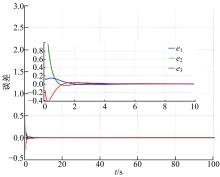
对于含有不确定参数c_i 的系统(12), (i=1, 2, 3, 4), q=0.95, r₁=r₂=r₃=0, 并且:

$\begin{matrix} [\begin{matrix} k_{1, 1} \\ k_{2, 1} \\ k_{3, 1} \end{matrix} \begin{matrix} k_{1, 2} \\ k_{2, 2} \\ k_{3, 2} \end{matrix} \begin{matrix} k_{1, 3} \\ k_{2, 3} \\ k_{3, 3} \end{matrix}] = [\begin{matrix} - 2 & - 1 & - 1 \\ - 3 & - 3 & - 1 \\ - 1 & - 2 & - 4 \end{matrix}] \end{matrix}$ 为负定。

其中, 初始状态 $\begin{matrix} (x_{1} (0), x_{2} (0), x_{3} (0)) = (0.1, 2, - 0.1), \end{matrix}$ 其自适应控制的系统误差曲线如图3所示。

	Figure Option View Download New Window
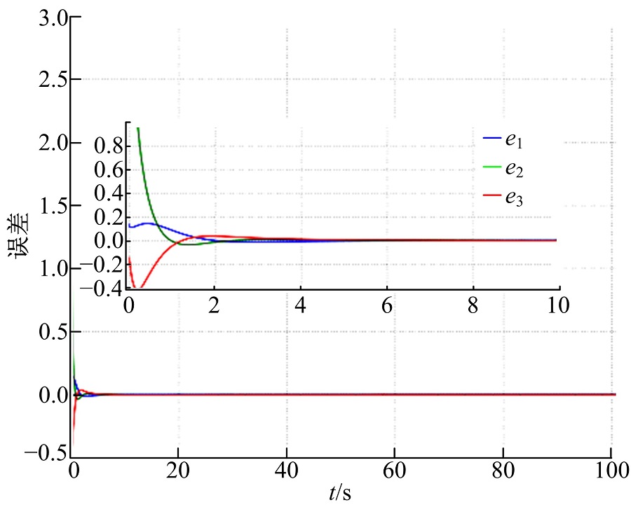	图3 自适应控制器的系统的误差曲线Fig.3 Error curves of system with adaptive controller

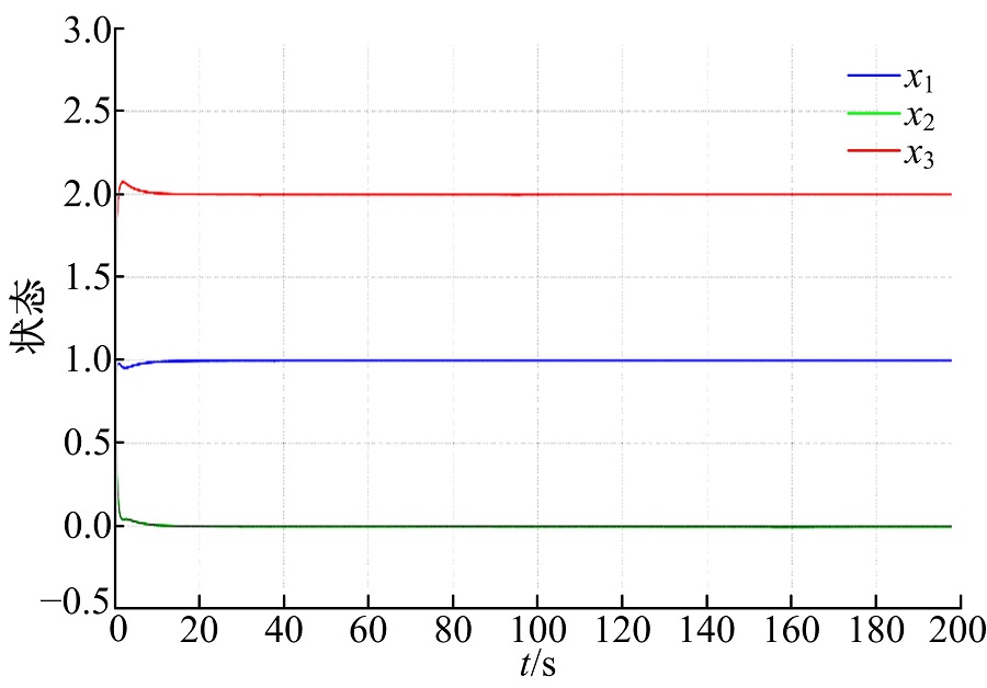当 $\begin{matrix} r_{1} = 2 、 r_{2} = 1 、 r_{3} = 0, \end{matrix}$ 其他参数不变时, 可得到图4所示的自适应控制的状态响应曲线, 图4表明状态变量完全追踪期望轨迹。

	Figure Option View Download New Window
	图4 自适应控制的状态响应Fig.4 States response with adaptive controller

本文设计了一种自适应控制器, 使系统状态变量追踪期望轨迹, 但追踪变量轨迹仍有待研究。

4 结束语

研究了一类无平衡点的混沌系统, 通过FDTM得到它的解集, 并分析了该系统的特点。通过判断最大Lyapunov特征指数, 给出了保持系统混沌的阶次范围。针对分数阶混沌系统设计出一种全状态自适应控制器, 可以用于追踪期望轨迹。最后, 通过数值模拟验证了本文方法的可行性。

The authors have declared that no competing interests exist.

参考文献

View Option

[1]	Meral F, Royston T, Magin R. Fractional calculus in viscoelasticity: an experimental study[J]. Communications in Nonlinear Science and Numerical Simulation, 2010, 15(4): 939-945. [本文引用:1]
[2]	Magin R L. Fractional calculus models of complex dynamics in biological tissues[J]. Computers & Mathematics with Applications, 2010, 59(5): 1586-1593. [本文引用:1]
[3]	Drapaca C, Sivaloganathan S. A fractional model of continuum mechanics[J]. Journal of Elasticity, 2012, 107(2) : 105-123. [本文引用:1]
[4]	Wiggins S. Introduction to Applied Nonlinear Dynamical Systems and Chaos[M]//Marsden J E, Sirovich L, Antman S S. Texts in Applied Mathematics. Berlin: Springer, 2003. [本文引用:1]
[5]	Hoppensteadt F C. Analysis and simulation of chaotic systems[J]. Journal of Applied Mathematics and Mechanics, 2002, 82(7): 472. [本文引用:1]
[6]	Li C, Peng G. Chaos in Chen's system with a fractional order[J]. Chaos, Solitons & Fractals, 2004, 22(2): 443-450. [本文引用:1]
[7]	Xu Y, Gu R, Zhang H, et al. Chaos in diffusionless lorenz system with a fractional order and its control[J]. International Journal of Bifurcation and Chaos, 2012, 22(4): 1250088. [本文引用:1]
[8]	Danca M F, Garrappa R. Suppressing chaos in discontinuous systems of fractional order by active control[J]. Applied Mathematics and Computation, 2015, 257: 89-102. [本文引用:1]
[9]	Tacha O I, Volos C K, Stouboulos I N, et al. Analysis, adaptive control and circuit simulation of a novel finance system with dissaving[J]. Archives of Control Sciences, 2016, 26(1): 95-115. [本文引用:1]
[10]	Kuntanapreeda S. Adaptive control of fractional-order unified chaotic systems using a passivity-based control approach[J]. Nonlinear Dynamics, 2016: 84(4): 2505-2515. [本文引用:1]
[11]	Wang Q, Zhang J, Ding D, et al. Adaptive mittag-leffler stabilization of a class of fractional order uncertain nonlinear systems[J]. Asian Journal of Control, 2016, 18(6): 2343-2351. [本文引用:1]
[12]	Arikoglu A, Ozkol I. Solution of fractional differential equations by using differential transform method[J]. Chaos, Solitons & Fractals, 2007, 34(5): 1473-1481. [本文引用:1]
[13]	Podlubny I. Fractional differential equations: an introduction to fractional derivatives, fractional differential equations, to methods of their solution and some of their applications[J]. Academic Press, 1999, 91(3): 427-436. [本文引用:1]
[14]	Odibat Z, Momani S. A generalized differential transform method for linear partial differential equations of fractional order[J]. Applied Mathematics Letters, 2008, 21(2): 194-199. [本文引用:1]
[15]	Eckmann J P, Kamphorst S O, Ruelle D, et al. Liapunov exponents from time series[J]. Physical Review A, 1986, 34(6): 4971-4979. [本文引用:1]
[16]	Takens F. Detecting Strange Attractors in Turbulence[M]//Smale S. Dynamical Systems and Turbulence. Berlin: Springer, 1981: 366-381. [本文引用:1]
[17]	Duarte-Mermoud M A, Aguila-Camacho N, Gallegos J A, et al. Using general quadratic Lyapunov functions to prove lyapunov uniform stability for fractional order systems[J]. Communications in Nonlinear Science and Numerical Simulation, 2015, 22(1): 650-659. [本文引用:1]
[18]	Li Y, Chen Y, Podlubny I. Mittag-leffler stability of fractional order nonlinear dynamic systems[J]. Automatica, 2009, 45(8): 1965-1969. [本文引用:1]
[19]	Li Y, Chen Y, Podlubny I. Stability of fractional-order nonlinear dynamic systems: Lyapunov direct method and generalized mittag-leffler stability[J]. Computers & Mathematics with Applications, 2010, 59(5): 1810-1821. [本文引用:1]
[20]	Caponetto R, Fazzino S. A semi-analytical method for the computation of the lyapunov exponents of fractional-order systems[J]. Communications in Nonlinear Science and Numerical Simulation, 2013, 18(1): 22-27. [本文引用:1]
[21]	Frederickson P, Kaplan J L, Yorke E D, et al. The Liapunov dimension of strange attractors[J]. Journal of Differential Equations, 1983, 49(2): 185-207. [本文引用:1]

2010

0.0

... 0 引言分数阶系统是包含分数阶积分与微分的动态系统,它可以有效地应用于物理系统建模^[1,2,3] ...

2010

0.0

... 0 引言分数阶系统是包含分数阶积分与微分的动态系统,它可以有效地应用于物理系统建模^[1,2,3] ...

2012

0.0

... 0 引言分数阶系统是包含分数阶积分与微分的动态系统,它可以有效地应用于物理系统建模^[1,2,3] ...

2003

0.0

... 在整数阶微积分的意义下,Poincare-Bendixon定理指出:连续自治系统出现混沌现象的微分阶次必须大于等于3^[4,5] ...

2002

0.0

... 在整数阶微积分的意义下,Poincare-Bendixon定理指出:连续自治系统出现混沌现象的微分阶次必须大于等于3^[4,5] ...

2004

0.0

... 但是,人们在研究中发现,在分数阶微积分的意义下,在许多阶次低于3的分数阶非线性系统中,仍然存在混沌现象^[6] ...

2012

0.0

... 文献^[7]提出了基于线性分数阶系统稳定性理论的混沌控制方法,然而这种方法只验证了局部的稳定性 ...

2015

0.0

... 文献^[8]提出了主动控制的方法,这种方法利用非线性控制律来消除控制系统中的非线性项,再根据线性分数阶系统稳定性理论,设计一个线性控制律来稳定此系统,但当系统中的参数未知时,不能用主动控制方法来设计控制器 ...

2016

0.0

... 文献^[9]研究了一类整数阶新型金融系统的自适应控制 ...

2016

0.0

... 文献^[10,11]研究了分数阶混沌系统的自适应控制,其中控制变量存在于局部系统方程中 ...

2016

0.0

... 文献^[10,11]研究了分数阶混沌系统的自适应控制,其中控制变量存在于局部系统方程中 ...

2007

0.0

... 1 预备知识本节给出了分数阶微积分和微分变换方法的一些定义和性质^[12] ...

1999

0.0

... Riemann-Liouville定义^[13],表示如下: ...

2008

0.0

... 以下是Caputo分数阶微分变换的基本性质^[14]:①如果f(t)=g(t)#cod#x000b1 ...

1986

0.0

... 对于分数阶系统来说,最常用的方法是用时间序列重构相空间,计算最大Lyapunov指数^[15],这种做法仍有很多缺点,如难以选择嵌入维数以及相空间重构的固有延迟参数^[16] ...

1981

0.0

2015

0.0

... 引理1^[17] 设 x(t)∈Rn是一个可微函数,对于任意 t≥0时,存在以下关系: ...

2009

0.0

... 定理1^[18,19] 设 x(t)=0为系统的一个平衡点,且: ...

2010

0.0

... 定理1^[18,19] 设 x(t)=0为系统的一个平衡点,且: ...

2013

0.0

... 利用文献^[20]中提到的方法,令L₁=0 ...

1983

0.0

... 根据Kaplan Yorke猜想,定义系统(9)的分数阶Lyapunov维数^[21]如下: ...